Introduction to Natural Language Processing (NLP) tools, frameworks, concepts, resources for Python
- spacy
- NLTK - similar to spacy, supports more models, simpl GUI model download
nltk.download() - gensim - topic modelling, accessing corpus, similarity calculations between query and indexed docs, SparseMatrixSimilarity, Latent Semantic Analysis
- lexnlp - information retrieval and extraction for real, unstructured legal text
- Holmes - information extraction, document classification, search in documents
- Pytorch-Transformers - includes BERT, GPT2, XLNet
Uncased model is better unless you know that case information is important for your task (e.g., Named Entity Recognition or Part-of-Speech tagging)
- PyTorch is an open source machine learning library based on the Torch library, used for applications such as computer vision and natural language processing
- Tensorflow
- Keras
- GPT-2 - generate fake news, text summaries
- BERT
- FinBERT - analyze sentiment of financial text
- XLnet
- ERNIE
- Gutenberg Corpus - contains 25,000 free electronic books.
from nltk.corpus import gutenberg - OntoNotes 5 - corpus comprising various genres of text (news, conversational telephone speech, weblogs, usenet newsgroups, broadcast, talk shows) in three languages (English, Chinese, and Arabic) with structural information (syntax and predicate argument structure) and shallow semantics (word sense linked to an ontology and coreference).
- wiki_en_tfidf.mm in gensim 3.9M documents, 100K features (distinct tokens) and 0.76G non-zero entries in the sparse TF-IDF matrix. The Wikipedia corpus contains about 2.24 billion tokens in total.
- GPT-2 Dataset
- Brown corpus - contains text from 500 sources, and the sources have been categorized by genre, such as news, editorial, and so on.
- Reuters Corpus - 10,788 news documents totaling 1.3 million words
- Newsfilter.io stock market news corpus - contains over 4 million press releases, earnings reports, FDA drug approvals, analyst ratings, merger agreements and many more covering all US companies listed on NASDAQ, NYSE, AMEX
- Kaggle - All the news, 143K articles
- Kaggle - Daily news for stock market prediction
- CNN News
- AG News - PyTorch integrated
spacy (good for beginners; use NLTK for bigger projects)
pip install spacy
python -m spacy download en
# python -m spacy download en_core_web_lg
LexNLP (good for dealing with legal and financial documents; installation guide here)
pip install https://github.com/LexPredict/lexpredict-lexnlp/archive/master.zip
python # to open REPL console
>>> import nltk
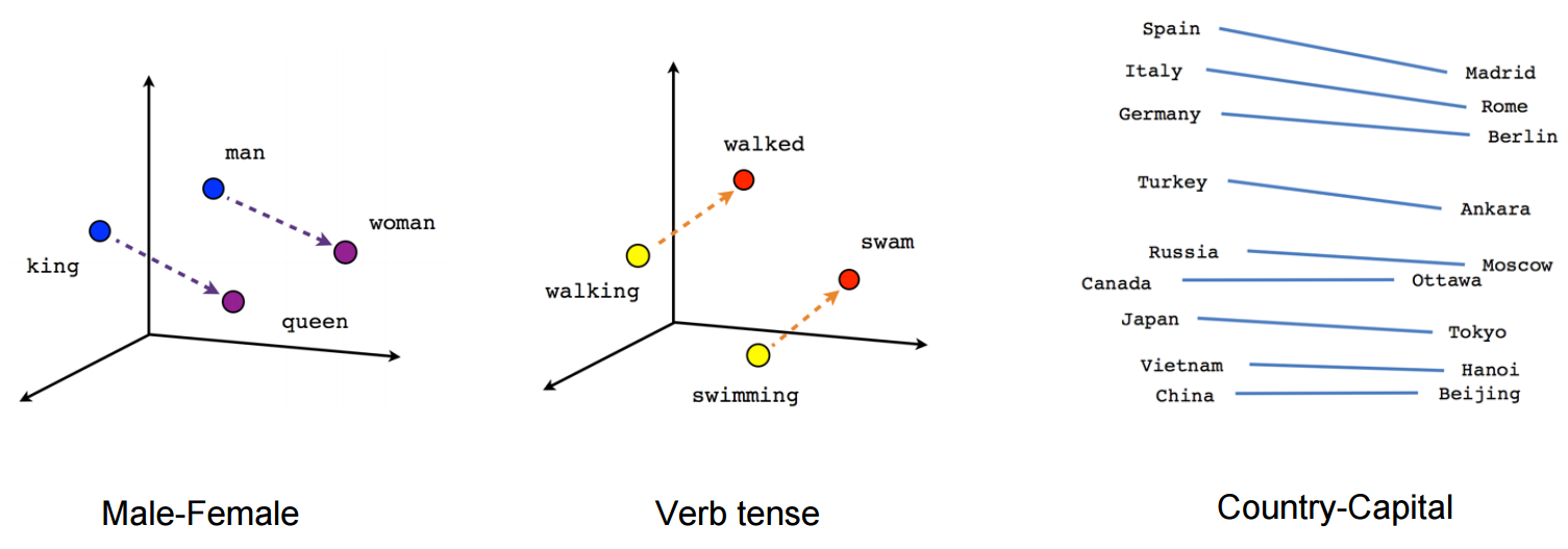
>>> nltk.download() # download all packagesVisualizing word vectors using PCA. Paper: https://papers.nips.cc/paper/5021-distributed-representations-of-words-and-phrases-and-their-compositionality.pdf
- Word embeddings are vector representation of words.
- Example sentence: word embeddings are words converted into numbers.
- A word in this sentence may be “Embeddings” or “numbers ” etc.
- A dictionary may be the list of all unique words in the sentence, eg [‘Word’,’Embeddings’,’are’,’Converted’,’into’,’numbers’]
- A vector representation of a word may be a one-hot encoded vector where 1 stands for the position where the word exists and 0 everywhere else.
- numbers = [0,0,0,0,0,1]
- converted = [0,0,0,1,0,0]
** Either use pre-trained word vectors or train our own**
- Word2Vec (Google, 2013), uses Skip Gram and CBOW
- Vectors trained on Google News (1.5GB) - vocabulary of 3 million words trained on around 100 billion words from the google news dataset
- GloVe (Stanford)
- Stanford Named Entity Recognizer (NER)
- LexPredict: pre-trained word embedding models for legal or regulatory text
- LexNLP legal models - US GAAP, finaical common terms, US federal regulators, common law
import gensim
word2vev_model = gensim.models.word2vec.Word2Vec(sentence_list)
https://www.analyticsvidhya.com/blog/2017/06/word-embeddings-count-word2veec/
- Count-based methods compute the statistics of how often some word co-occurs with its neighbor words in a large text corpus, and then map these count-statistics down to a small, dense vector for each word.
- Predictive models directly try to predict a word from its neighbors in terms of learned small, dense embedding vectors (considered parameters of the model).
- Example: Word2vec (Google)
Term Frequency - Inverse Document Frequency
- Term frequency equals the number of times a word appears in a document divided by the total number of words in the document.
- Inverse document frequency calculates the weight of rare words in all documents in the corpus, with rare words having a high IDF score, and words that are present in all documents in a corpus having IDF close to zero.
(sklearn) in Python has a function TfidfVectorizer() that will compute the TF-IDF values for you
from sklearn.feature_extraction.text import TfidfVectorizer
# Write a function for cleaning strings and returning an array of ngrams
def ngrams_analyzer(string):
    string = re.sub(r'[,-./]', r'', string)
    ngrams = zip(*[string[i:] for i in range(5)])  # N-Gram length is 5
    return [''.join(ngram) for ngram in ngrams]
# Construct your vectorizer for building the TF-IDF matrix
vectorizer = TfidfVectorizer(analyzer=ngrams_analyzer)
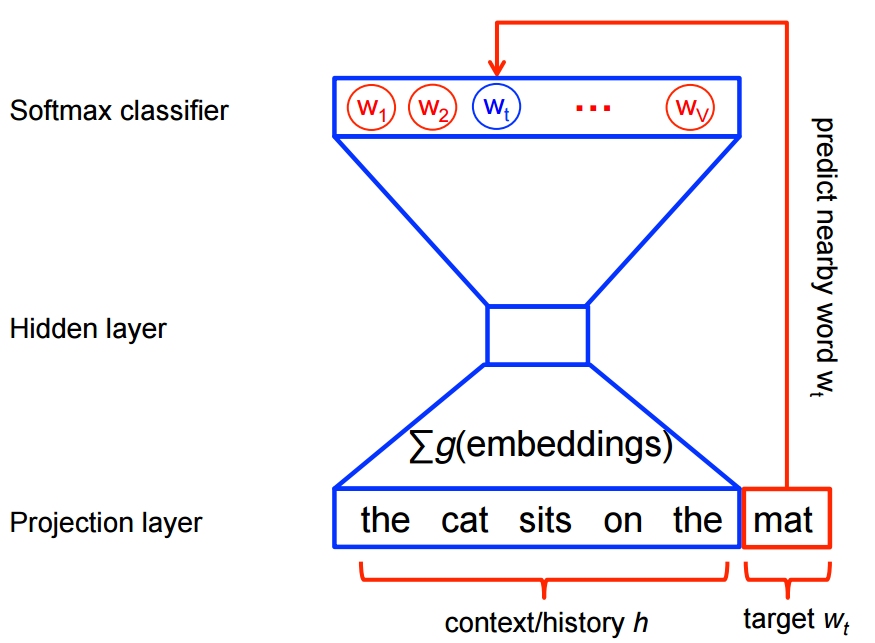
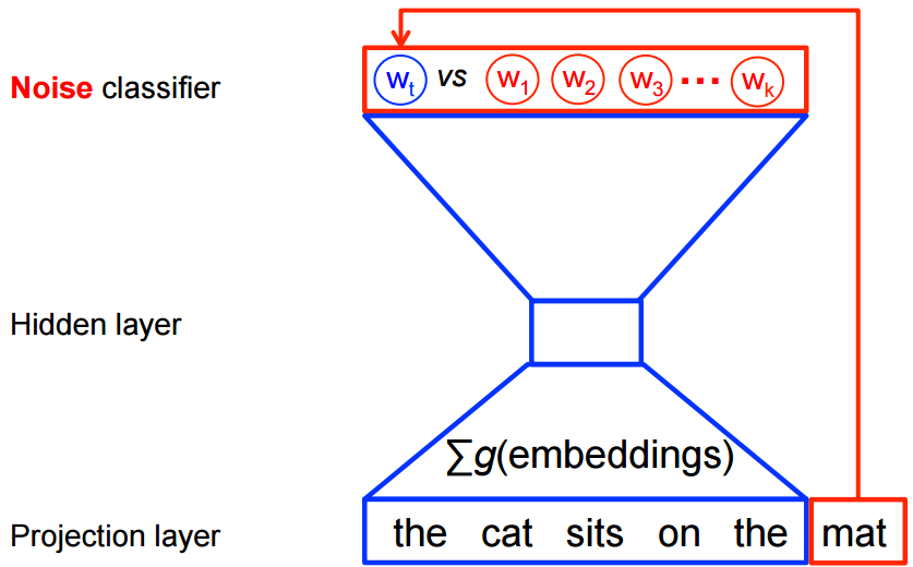
# Credits: https://towardsdatascience.com/group-thousands-of-similar-spreadsheet-text-cells-in-seconds-2493b3ce6d8d- Uses Neural Networks
- CBOW predicts target words (e.g. 'mat') from source context words ('the cat sits on the')
- Skip-gram does the inverse and predicts source context-words from the target words
Skip – gram follows the same topology as of CBOW. It just flips CBOW’s architecture on its head. The aim of skip-gram is to predict the context given a word
# John likes to watch movies. Mary likes movies too.
BoW1 = {"John":1,"likes":2,"to":1,"watch":1,"movies":2,"Mary":1,"too":1};import spacy# Import dataset
nlp = spacy.load("en")
# Import large dataset. Needs to be downloaded first.
# nlp = spacy.load("en_core_web_lg")Stop words are the very common words like ‘if’, ‘but’, ‘we’, ‘he’, ‘she’, and ‘they’. We can usually remove these words without changing the semantics of a text and doing so often (but not always) improves the performance of a model.
# spacy: Removing stop words
spacy_stopwords = spacy.lang.en.stop_words.STOP_WORDS
print('spacy: Number of stop words: %d' % len(spacy_stopwords))
spacy: Number of stop words: 326
# nltk: Removing stop words
from nltk.corpus import stopwords
english_stop_words = stopwords.words('english')
print('ntlk: Number of stop words: %d' % len(english_stop_words))
ntlk: Number of stop words: 179
text = 'Larry Page founded Google in early 1990.'
doc = nlp(text)
tokens = [token.text for token in doc if not token.is_stop]
print('Original text: %s' % (text))
print()
print(tokens)
Original text: Larry Page founded Google in early 1990.
['Larry', 'Page', 'founded', 'Google', 'early', '1990', '.']
Part of a given text. So doc[2:4] is a span starting at token 2, up to – but not including! – token 4.
Docs: https://spacy.io/api/span
doc = nlp("Larry Page founded Google in early 1990.")
span = doc[2:4]
span.text
'founded Google'
[(spans) for spans in doc][Larry, Page, founded, Google, in, early, 1990, .]
Segmenting text into words, punctuation etc.
- Sentence tokenization
- Word tokenization
Docs: https://spacy.io/api/token
doc = nlp("Larry Page founded Google in early 1990.")
[token.text for token in doc]
['Larry', 'Page', 'founded', 'Google', 'in', 'early', '1990', '.']
# Load OpenAI GPT-2 using PyTorch Transformers
tokenizer = GPT2Tokenizer.from_pretrained('gpt2')
model = GPT2Model.from_pretrained('gpt2')
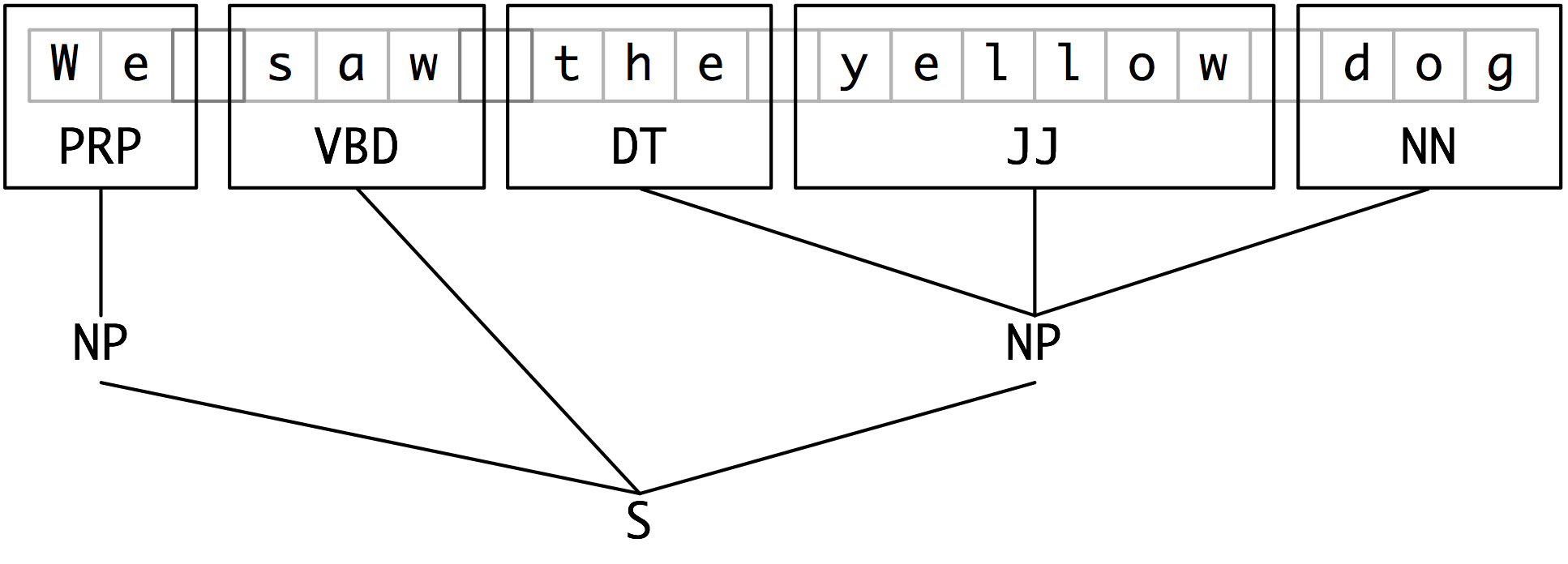
# https://huggingface.co/pytorch-transformers/serialization.htmlSegments and labels multi-token sequences.
- Each of these larger boxes is called a chunk.
- Like tokenization, which omits whitespace, chunking usually selects a subset of the tokens.
- The pieces produced by a chunker do not overlap in the source text.
Credits: https://www.nltk.org/book/ch07.html
Chink is a sequence of tokens that is not included in a chunk.
Credits: https://www.nltk.org/book/ch07.html
Assigning word types to tokens like verb or noun.
POS tagging should be done straight after tokenization and before any words are removed so that sentence structure is preserved and it is more obvious what part of speech the word belongs to.
text = "Asian shares skidded on Tuesday after a rout in tech stocks put Wall Street to the sword"
doc = nlp(text)
[(x.orth_, x.pos_, spacy.explain(x.pos_)) for x in [token for token in doc]]
[('Asian', 'ADJ', 'adjective'),
('shares', 'NOUN', 'noun'),
('skidded', 'VERB', 'verb'),
('on', 'ADP', 'adposition'),
('Tuesday', 'PROPN', 'proper noun'),
('after', 'ADP', 'adposition'),
('a', 'DET', 'determiner'),
('rout', 'NOUN', 'noun'),
('in', 'ADP', 'adposition'),
('tech', 'NOUN', 'noun'),
('stocks', 'NOUN', 'noun'),
('put', 'VERB', 'verb'),
('Wall', 'PROPN', 'proper noun'),
('Street', 'PROPN', 'proper noun'),
('to', 'ADP', 'adposition'),
('the', 'DET', 'determiner'),
('sword', 'NOUN', 'noun')]
[(x.orth_, x.tag_, spacy.explain(x.tag_)) for x in [token for token in doc]][('Asian', 'JJ', 'adjective'),
('shares', 'NNS', 'noun, plural'),
('skidded', 'VBD', 'verb, past tense'),
('on', 'IN', 'conjunction, subordinating or preposition'),
('Tuesday', 'NNP', 'noun, proper singular'),
('after', 'IN', 'conjunction, subordinating or preposition'),
('a', 'DT', 'determiner'),
('rout', 'NN', 'noun, singular or mass'),
('in', 'IN', 'conjunction, subordinating or preposition'),
('tech', 'NN', 'noun, singular or mass'),
('stocks', 'NNS', 'noun, plural'),
('put', 'VBD', 'verb, past tense'),
('Wall', 'NNP', 'noun, proper singular'),
('Street', 'NNP', 'noun, proper singular'),
('to', 'IN', 'conjunction, subordinating or preposition'),
('the', 'DT', 'determiner'),
('sword', 'NN', 'noun, singular or mass')]
# using nltk
import nltk
tokens = nltk.word_tokenize(text)
pos_tags = nltk.pos_tag(tokens)
pos_tags
[('Asian', 'JJ'),
('shares', 'NNS'),
('skidded', 'VBN'),
('on', 'IN'),
('Tuesday', 'NNP'),
('after', 'IN'),
('a', 'DT'),
('rout', 'NN'),
('in', 'IN'),
('tech', 'JJ'),
('stocks', 'NNS'),
('put', 'VBD'),
('Wall', 'NNP'),
('Street', 'NNP'),
('to', 'TO'),
('the', 'DT'),
('sword', 'NN')]
- BEGIN - The first token of a multi-token entity.
- IN - An inner token of a multi-token entity.
- LAST - The final token of a multi-token entity.
- UNIT - A single-token entity.
- OUT - A non-entity token.
[(token, token.ent_iob_, token.ent_type_) for token in doc][(Asian, 'B', 'NORP'),
(shares, 'O', ''),
(skidded, 'O', ''),
(on, 'O', ''),
(Tuesday, 'B', 'DATE'),
(after, 'O', ''),
(a, 'O', ''),
(rout, 'O', ''),
(in, 'O', ''),
(tech, 'O', ''),
(stocks, 'O', ''),
(put, 'O', ''),
(Wall, 'O', ''),
(Street, 'O', ''),
(to, 'O', ''),
(the, 'O', ''),
(sword, 'O', '')]
Stemming is the process of reducing words to their root form.
Examples:
- cats, catlike, catty → cat
- fishing, fished, fisher → fish
There are two types of stemmers in NLTK: Porter Stemmer and Snowball stemmers
import nltk
from nltk.stem.porter import *
stemmer = PorterStemmer()
tokens = ['compute', 'computer', 'computed', 'computing']
for token in tokens:
    print(token + ' --> ' + stemmer.stem(token))
compute --> comput
computer --> comput
computed --> comput
computing --> comput
Assigning the base form of word, for example:
- "was" → "be"
- "rats" → "rat"
doc = nlp("Was Google founded in early 1990?")
[(x.orth_, x.lemma_) for x in [token for token in doc]]
[('Was', 'be'),
('Google', 'Google'),
('founded', 'found'),
('in', 'in'),
('early', 'early'),
('1990', '1990'),
('?', '?')]
Finding and segmenting individual sentences.
doc = nlp("Larry Page founded Google in early 1990. Sergey Brin joined.")
[sent.text for sent in doc.sents]
['Larry Page founded Google in early 1990.', 'Sergey Brin joined.']
Assigning syntactic dependency labels, describing the relations between individual tokens, like subject or object.
doc = nlp("We are reading a text.")
# Dependency labels
[(x.orth_, x.dep_, spacy.explain(x.dep_)) for x in [token for token in doc]]
[('We', 'nsubj', 'nominal subject'),
('are', 'aux', 'auxiliary'),
('reading', 'ROOT', None),
('a', 'det', 'determiner'),
('text', 'dobj', 'direct object'),
('.', 'punct', 'punctuation')]
# Syntactic head token (governor)
[token.head.text for token in doc]
['reading', 'reading', 'reading', 'text', 'reading', 'reading']
doc = nlp("I have a red car")
[chunk.text for chunk in doc.noun_chunks]
['I', 'a red car']
What is NER? Labeling "real-world" objects, like persons, companies or locations.
2 popular approaches:
- Rule-based
- ML-based:
- Multi-class classification
- Conditional Random Field (probabilistic graphical model)
Datasets:
Credits: https://medium.com/@yingbiao/ner-with-bert-in-action-936ff275bc73
Entities supported by spacy:
- PERSON People, including fictional.
- NORP Nationalities or religious or political groups.
- FAC Buildings, airports, highways, bridges, etc.
- ORG Companies, agencies, institutions, etc.
- GPE Countries, cities, states.
- LOC Non-GPE locations, mountain ranges, bodies of water.
- PRODUCT Objects, vehicles, foods, etc. (Not services.)
- EVENT Named hurricanes, battles, wars, sports events, etc.
- WORK_OF_ART Titles of books, songs, etc.
- LAW Named documents made into laws.
- LANGUAGE Any named language.
- DATE Absolute or relative dates or periods.
- TIME Times smaller than a day.
- PERCENT Percentage, including ”%“.
- MONEY Monetary values, including unit.
- QUANTITY Measurements, as of weight or distance.
- ORDINAL “first”, “second”, etc.
- CARDINAL Numerals that do not fall under another type.
LexNLP entities:
- acts, e.g., “section 1 of the Advancing Hope Act, 1986”
- amounts, e.g., “ten pounds” or “5.8 megawatts”
- citations, e.g., “10 U.S. 100” or “1998 S. Ct. 1”
- companies, e.g., “Lexpredict LLC”
- conditions, e.g., “subject to …” or “unless and until …”
- constraints, e.g., “no more than” or “
- copyright, e.g., “(C) Copyright 2000 Acme”
- courts, e.g., “Supreme Court of New York”
- CUSIP, e.g., “392690QT3”
- dates, e.g., “June 1, 2017” or “2018-01-01”
- definitions, e.g., “Term shall mean …”
- distances, e.g., “fifteen miles”
- durations, e.g., “ten years” or “thirty days”
- geographic and geopolitical entities, e.g., “New York” or “Norway”
- money and currency usages, e.g., “$5” or “10 Euro”
- percents and rates, e.g., “10%” or “50 bps”
- PII, e.g., “212-212-2121” or “999-999-9999”
- ratios, e.g.,” 3:1” or “four to three”
- regulations, e.g., “32 CFR 170”
- trademarks, e.g., “MyApp (TM)”
- URLs, e.g., “http://acme.com/”
Stanford NER entities:
- Location, Person, Organization, Money, Percent, Date, Time
NLTK
- NLTK maximum entropy classifier
doc = nlp("Larry Page founded Google in the US in early 1990.")
# Text and label of named entity span
[(ent.text, ent.label_) for ent in doc.ents]
[('Larry Page', 'PERSON'),
('Google', 'ORG'),
('US', 'GPE'),
('early 1990', 'DATE')]
doc = nlp('European authorities fined Google a record $5.1 billion on Wednesday for abusing its power in the mobile phone market and ordered the company to alter its practices')
[(X.text, X.label_) for X in doc.ents]
[('European', 'NORP'),
('Google', 'ORG'),
('$5.1 billion', 'MONEY'),
('Wednesday', 'DATE')]
from collections import Counter
labels = [x.label_ for x in doc.ents]
Counter(labels)
Counter({'NORP': 1, 'ORG': 1, 'MONEY': 1, 'DATE': 1})
[(X, X.ent_iob_, X.ent_type_) for X in doc][(European, 'B', 'NORP'),
(authorities, 'O', ''),
(fined, 'O', ''),
(Google, 'B', 'ORG'),
(a, 'O', ''),
(record, 'O', ''),
($, 'B', 'MONEY'),
(5.1, 'I', 'MONEY'),
(billion, 'I', 'MONEY'),
(on, 'O', ''),
(Wednesday, 'B', 'DATE'),
(for, 'O', ''),
(abusing, 'O', ''),
(its, 'O', ''),
(power, 'O', ''),
(in, 'O', ''),
(the, 'O', ''),
(mobile, 'O', ''),
(phone, 'O', ''),
(market, 'O', ''),
(and, 'O', ''),
(ordered, 'O', ''),
(the, 'O', ''),
(company, 'O', ''),
(to, 'O', ''),
(alter, 'O', ''),
(its, 'O', ''),
(practices, 'O', '')]
# Show Begin and In entities
items = [x.text for x in doc.ents]
print(items)
Counter(items).most_common(3)
['European', 'Google', '$5.1 billion', 'Wednesday']
[('European', 1), ('Google', 1), ('$5.1 billion', 1)]
import lexnlp.extract.en as lexnlp
import nltk
text = "There are ten cows in the 2 acre pasture."
print(list(lexnlp.amounts.get_amounts(text)))[10, 2.0]
import lexnlp.extract.en.acts
text = "test section 12 of the VERY Important Act of 1954."
lexnlp.extract.en.acts.get_act_list(text)
[{'location_start': 5,
'location_end': 49,
'act_name': 'VERY Important Act',
'section': '12',
'year': '1954',
'ambiguous': False,
'value': 'section 12 of the VERY Important Act of 1954'}]
Two types:
- binary classification (text only belongs to one class)
- multi-class classification (text can belong to multiple classes)
Assigning categories or labels to a whole document, or parts of a document.
Approach:
- calculate document vectors for each document
- use kNN to calculate clusters based on document vectors
- each cluster represents a class of documents that are similar to each other
# Credits: https://pytorch.org/tutorials/beginner/text_sentiment_ngrams_tutorial.html
import re
from torchtext.data.utils import ngrams_iterator
from torchtext.data.utils import get_tokenizer
ag_news_label = {1 : "World",
                 2 : "Sports",
                 3 : "Business",
                 4 : "Sci/Tec"}
def predict(text, model, vocab, ngrams):
    tokenizer = get_tokenizer("basic_english")
    with torch.no_grad():
        text = torch.tensor([vocab[token]
                            for token in ngrams_iterator(tokenizer(text), ngrams)])
        output = model(text, torch.tensor([0]))
        return output.argmax(1).item() + 1
ex_text_str = "MEMPHIS, Tenn. – Four days ago, Jon Rahm was \
    enduring the season’s worst weather conditions on Sunday at The \
    Open on his way to a closing 75 at Royal Portrush, which \
    considering the wind and the rain was a respectable showing. \
    Thursday’s first round at the WGC-FedEx St. Jude Invitational \
    was another story. With temperatures in the mid-80s and hardly any \
    wind, the Spaniard was 13 strokes better in a flawless round. \
    Thanks to his best putting performance on the PGA Tour, Rahm \
    finished with an 8-under 62 for a three-stroke lead, which \
    was even more impressive considering he’d never played the \
    front nine at TPC Southwind."
vocab = train_dataset.get_vocab()
model = model.to("cpu")
print("This is a %s news" %ag_news_label[predict(ex_text_str, model, vocab, 2)])
# Output: This is a Sports news- Convert a collection of text documents to a matrix of token counts
- skikitLearn
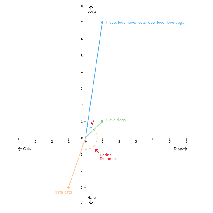
How similar are two documents, sentences, token or spans? Cosine similarity (also known as: L2-normalized dot product of vectors) is a formula used to calculate how similar two given word vectors are. How to calculate Cosine similarity?
- spacy (see example below)
- scikit: sklearn.metrics.pairwise.cosine_similarity
Figure below shows three word vectors and Cosine distance (=similarity) between
- "I hate cats" and "I love dogs" (result: not very similar)
- "I love dogs" and "I love, love, love, .. dogs" (result: similar)
ModuleNotFoundError: No module named 'Levenshtein'
- State -> action -> state -> action ...
- Agent
- Set of actions
- Transitions
- Discount factor
- Reward

A measure of how far a model's predictions are from its label. In contrast to:
- reward function
Mean Squared Error (MSE) is a common loss function used for regression problems. Mean squared error of an estimator measures the average of the squares of the errors—that is, the average squared difference between the estimated values and the actual value. Can be used for regression problems (say, to predict the price of a house). Alternatives:
- Binary Crossentropy Loss (is better for dealing with probabilities)
Used in binary classification tasks, ie model outputs a probability (a single-unit layer with a sigmoid activation), we'll use the binary_crossentropy loss function.
Used in image classification task
Used in logistic regression tasks
This is how the model is updated based on the data it sees and its loss function.
Optimization algorithm for finding the minimum of a function.
- Keras (best learning tool for beginners)
- PyTorch (dynamic)
- Tensorflow (declerative programming, can run on Apache Spark)
- Binary
- Not binary
A function (for example, ReLU or sigmoid) that takes in the weighted sum of all of the inputs from the previous layer and then generates and passes an output value (typically nonlinear) to the next layer. https://developers.google.com/machine-learning/glossary/#activation_function
A function that provides probabilities for each possible class in a multi-class classification model. The probabilities add up to exactly 1.0. For example, softmax might determine that the probability of a particular image being a dog at 0.9, a cat at 0.08, and a horse at 0.02. Example: last layer is a 10-node softmax layer—this returns an array of 10 probability scores that sum to 1.
A function that maps logistic or multinomial regression output (log odds) to probabilities, returning a value between 0 and 1 Sigmoid function converts /sigma into a probability between 0 and 1.
- If input is negative or zero, output is 0.
- If input is positive, output is equal to input.
Used when taining a neural network.
TP/(TP+FP)
- TP=true positive
- FP=false positive
TP/(TP+FN)
(2 × Precision × Recall) / (Precision + Recall)
A common regression metric is Mean Absolute Error (MAE).
Early stopping is a useful technique to prevent overfitting.
penalizes weights in proportion to the sum of the absolute values of the weights https://developers.google.com/machine-learning/glossary/#L1_regularization
penalizes weights in proportion to the sum of the squares of the weights
The number of elements set to zero (or null) in a vector or matrix divided by the total number of entries in that vector or matrix.
Used by Reddit to rank comments.
https://spacy.io/models/en#en_pytt_xlnetbasecased_lg
A confusion matrix is a table where each cell [i,j] indicates how often label j was predicted when the correct label was i.
- Every feature gets a say in determining which label should be assigned to a given input value.
- To choose a label for an input value, the naive Bayes classifier begins by calculating the prior probability of each label, which is determined by checking frequency of each label in the training set. Credits: https://www.nltk.org/book/ch06.html
