Random forest submission one
In the last version of this notebook, tried to improve our score by doing some simple feature selection on the f
import matplotlib
import matplotlib.pyplot as plt
import numpy as np


%matplotlib inline
plt.rcParams['figure.figsize'] = 6, 4.5
plt.rcParams['axes.grid'] = True
plt.gray()


<matplotlib.figure.Figure at 0x7fea12328080>
As before, loading the data. But, now there's more data to load.
cd ..

/home/gavin/repositories/hail-seizure


import train
import json
import imp


settings = json.load(open('SETTINGS.json', 'r'))


settings['FEATURES']


['ica_feat_var_',
 'ica_feat_cov_',
 'ica_feat_corrcoef_',
 'ica_feat_pib_',
 'ica_feat_xcorr_',
 'ica_feat_psd_',
 'ica_feat_psd_logf_',
 'ica_feat_coher_',
 'ica_feat_coher_logf_',
 'raw_feat_var_',
 'raw_feat_cov_',
 'raw_feat_corrcoef_',
 'raw_feat_pib_',
 'raw_feat_xcorr_',
 'raw_feat_psd_',
 'raw_feat_psd_logf_',
 'raw_feat_coher_',
 'raw_feat_coher_logf_']


data = train.get_data(settings['FEATURES'])


!free -m

             total       used       free     shared    buffers     cached
Mem:         11933      11736        196         62         48       3061
-/+ buffers/cache:       8626       3306
Swap:        12287       1041      11246
It's not generally a good idea to run anything that's going to take a long time in an IPython notebook. The thing can freeze, or if it's disconnected lose work. Going to develop a script here that can be run locally or on salmon.
# getting a set of the subjects involved
subjects = set(list(data.values())[0].keys())
print(subjects)

{'Dog_5', 'Patient_2', 'Patient_1', 'Dog_2', 'Dog_4', 'Dog_1', 'Dog_3'}


import sklearn.preprocessing
import sklearn.pipeline
import sklearn.ensemble
import sklearn.cross_validation
from train import utils
We want to do some simple feature selection, as even with a massive amount of RAM available there's no point in using features that are obviously useless. The first suggestion for this is a variance threshold, removing features with low variances.
X,y = utils.build_training(list(subjects)[0],list(data.keys()),data)


h=plt.hist(np.log10(np.var(X,axis=0)))
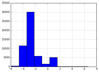
However, I don't really like this much, as low variance doesn't mean that there won't be information there. After all, variance scales with the multiplicative constants.
A better approach is scikit-learns SelectKBest, which can use
import sklearn.feature_selection


Xbest = sklearn.feature_selection.SelectKBest(sklearn.feature_selection.f_classif, k=50).fit_transform(X,y)


import sklearn.decomposition


pca = sklearn.decomposition.PCA(n_components=2)
scaler = sklearn.preprocessing.StandardScaler()
twodX = pca.fit_transform(scaler.fit_transform(Xbest))
plt.scatter(twodX[:,0][y==1],twodX[:,1][y==1],c='blue')
plt.scatter(twodX[:,0][y==0],twodX[:,1][y==0],c='red')


<matplotlib.collections.PathCollection at 0x7fe929030518>
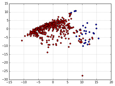
Looking good, now doing the same with the magical t-SNE:
import sklearn.manifold


tsne = sklearn.manifold.TSNE()
twodX = tsne.fit_transform(scaler.fit_transform(Xbest))
plt.scatter(twodX[:,0][y==1],twodX[:,1][y==1],c='blue')
plt.scatter(twodX[:,0][y==0],twodX[:,1][y==0],c='red')


<matplotlib.collections.PathCollection at 0x7fe928042d30>
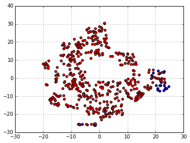
Also looking good.
So, all we do is add the selection to our model and then also turn the
n_estimators up and we should get a better prediction.
selection = sklearn.feature_selection.SelectKBest(sklearn.feature_selection.f_classif,k=3000)
scaler = sklearn.preprocessing.StandardScaler()
forest = sklearn.ensemble.RandomForestClassifier()
model = sklearn.pipeline.Pipeline([('sel',selection),('scl',scaler),('clf',forest)])
Testing this model on this single subject:
def subjpredictions(subject,model,data):
    X,y = utils.build_training(subject,list(data.keys()),data)
    cv = sklearn.cross_validation.StratifiedShuffleSplit(y)
    predictions = []
    labels = []
    allweights = []
    for train,test in cv:
        # calculate weights
        weight = len(y[train])/sum(y[train])
        weights = np.array([weight if i == 1 else 1 for i in y[train]])
        model.fit(X[train],y[train],clf__sample_weight=weights)
        predictions.append(model.predict_proba(X[test]))
        weight = len(y[test])/sum(y[test])
        weights = np.array([weight if i == 1 else 1 for i in y[test]])
        allweights.append(weights)
        labels.append(y[test])
    predictions = np.vstack(predictions)[:,1]
    labels = np.hstack(labels)
    weights = np.hstack(allweights)
    return predictions,labels,weights


p,l,w = subjpredictions(list(subjects)[0],model,data)


sklearn.metrics.roc_auc_score(l,p)


0.96511111111111114


fpr,tpr,thresholds = sklearn.metrics.roc_curve(l,p)
plt.plot(fpr,tpr)


[<matplotlib.lines.Line2D at 0x7fe928034518>]
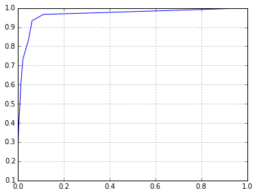
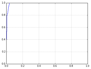
It certainly works a bit better than the classifier I was working with before. What if we increase the number of estimators to deal with the much larger number of features?
model.set_params(clf__n_estimators=5000)


Pipeline(steps=[('sel', SelectKBest(k=3000, score_func=<function f_classif at 0x7fe939067730>)), ('scl', StandardScaler(copy=True, with_mean=True, with_std=True)), ('clf', RandomForestClassifier(bootstrap=True, compute_importances=None,
            criterion='gini', max_depth=None, max_features='auto',
            max_leaf_nodes=None, min_density=None, min_samples_leaf=1,
            min_samples_split=2, n_estimators=5000, n_jobs=1,
            oob_score=False, random_state=None, verbose=0))])


%%time
p,l,w = subjpredictions(list(subjects)[0],model,data)

CPU times: user 2min 30s, sys: 36.3 s, total: 3min 6s
Wall time: 3min 6s


sklearn.metrics.roc_auc_score(l,p)


0.99296296296296305


fpr,tpr,thresholds = sklearn.metrics.roc_curve(l,p)
plt.plot(fpr,tpr)


[<matplotlib.lines.Line2D at 0x7fe927f4ecc0>]
Actually, it looks like I could probably just run this in the notebook, and it'd probably be fine. Will write the script after doing this.
features = list(data.keys())


%%time
predictiondict = {}
for subj in subjects:
    # training step
    X,y = utils.build_training(subj,features,data)
    # weights
    weight = len(y)/sum(y)
    weights = np.array([weight if i == 1 else 1 for i in y])
    model.fit(X,y,clf__sample_weight=weights)
    # prediction step
    X,segments = utils.build_test(subj,features,data)
    predictions = model.predict_proba(X)
    for segment,prediction in zip(segments,predictions):
        predictiondict[segment] = prediction

/home/gavin/.local/lib/python3.4/site-packages/sklearn/feature_selection/univariate_selection.py:106: RuntimeWarning: invalid value encountered in true_divide
  f = msb / msw
/home/gavin/.local/lib/python3.4/site-packages/sklearn/feature_selection/univariate_selection.py:106: RuntimeWarning: invalid value encountered in true_divide
  f = msb / msw


CPU times: user 5min 48s, sys: 1min 1s, total: 6min 50s
Wall time: 8min 22s


/home/gavin/.local/lib/python3.4/site-packages/sklearn/feature_selection/univariate_selection.py:106: RuntimeWarning: invalid value encountered in true_divide
  f = msb / msw


import csv


with open("output/protosubmission.csv","w") as f:
    c = csv.writer(f)
    c.writerow(['clip','preictal'])
    for seg in predictiondict.keys():
        c.writerow([seg,"%s"%predictiondict[seg][-1]])
Submitting now, and got approximately 0.4, worse than all zeros. How did that happen? Something to do with the warnings above, possibly?
Checking if there's anything obviously weird with the output file:
!head output/protosubmission.csv
Nope, looks ok.
There are three warnings above, so this problem is only occurring on three of the subjects. Could run each subject individually and try to find one where the ROC completely falls apart.
%%time
for s in subjects:
    p,l,w = subjpredictions(s,model,data)
    print("subject %s"%s, sklearn.metrics.roc_auc_score(l,p,sample_weight=w))
Simple solution is apparently to [run a variance threshold](https://github.com /scikit-learn/scikit-learn/issues/3624) before running the feature selection (like it says on the wiki really).
thresh = sklearn.feature_selection.VarianceThreshold()
selection = sklearn.feature_selection.SelectKBest(sklearn.feature_selection.f_classif,k=3000)
scaler = sklearn.preprocessing.StandardScaler()
forest = sklearn.ensemble.RandomForestClassifier()
model = sklearn.pipeline.Pipeline([('thr',thresh),('sel',selection),('scl',scaler),('clf',forest)])


%%time
predictiondict = {}
for subj in subjects:
    # training step
    X,y = utils.build_training(subj,features,data)
    # weights
    weight = len(y)/sum(y)
    weights = np.array([weight if i == 1 else 1 for i in y])
    model.fit(X,y,clf__sample_weight=weights)
    # prediction step
    X,segments = utils.build_test(subj,features,data)
    predictions = model.predict_proba(X)
    for segment,prediction in zip(segments,predictions):
        predictiondict[segment] = prediction

CPU times: user 2min 14s, sys: 47 s, total: 3min 1s
Wall time: 4min 58s


with open("output/protosubmission.csv","w") as f:
    c = csv.writer(f)
    c.writerow(['clip','preictal'])
    for seg in predictiondict.keys():
        c.writerow([seg,"%s"%predictiondict[seg][-1]])